Option Strategies
Introduction
Options are the most versatile trading tool today. No other investment vehicle seems to have a unique set of characteristics and flexibility that options provide to a trader.
It gives investors and traders a lot of efficient ways to strategise their trades efficiently achieving better risk rewards to their trades. Options can help the traders in volatile and unpredictable markets by enabling them to profit in numerous ways.
One of the reasons why traders are lured to option trading is they can generate returns exceeding 100% and sometimes even 1000% in a short time frame.
On the contrary, trading options without proper knowledge is a bad idea! They can expire worthless after a set time frame at which their entire value is worthless. Correct application of when to hold options, when to allow them expire or when to exercise is important for every trader to know before they trade. But why should anyone trade in options? Let us understand in the next unit.
Why Trade Options?
Options being the most versatile instrument in the derivative segment helps the traders in many ways.
It is used to manage risk, generate income, leverage the existing trades and make profits under almost all types of market conditions.
Options can enable the traders to speculate on the asset when it is expected to rise, fall, or move sideways within a selected time frame.
With options, one can engage with limited or unlimited risk. The versatility of options, in combination with leverage, is what makes it different from other trading vehicles.
The key to success while trading with options is to first determine your view on the stock and simultaneously the time frame and then determine the option strategy that can meet that perspective.
Let me list down some reasons why Options are every trader's favourite!
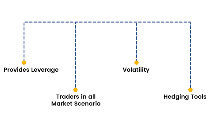
Leverage
An option contract helps a trader leverage their position to a great extent. It involves paying up a cost that is usually a small fraction of the cost of what he or she would pay for an equivalent number of shares otherwise.
The cost basis is very low when trading options. The position is much more sensitive to the underlying stock's price movements, and hence the percentage returns can be much greater.
Trade in every market scenario
Options help you generate income from almost all market situations. Traders make profits from trending stocks. Traders use puts and calls to ensure that you can make money if the stock goes up, down, or even sideways.
Volatility
Different options strategies protect or enable the traders to benefit from factors such as time decay, volatility, lack of volatility, and more. A correct reading and assessment of volatility can take you a long way in generating constant profits.
Hedging Tool
Options are a great hedging tool. It enables you to substantially reduce your risk of trading, or even eliminate risk altogether with certain hedging strategies.
So, with all the different benefits of options, why on earth would traders not be eager to learn more about them?
Option Chain
In this section, we are going to learn an extremely useful tool that provides a listing of all available options contracts called ‘Option Chain’.
What is the Option chain?
Option chain is an integral tool to every option trader. It is a matrix where all the option contracts -both call and puts are listed in a chronological order.
Traders use the option chain to understand the dynamics and the direction of price movements. It also helps to identify which options contracts are liquid and which are illiquid. Normally it helps the traders to evaluate the depth and liquidity of specific strikes. An Option chain helps a trader with the following information and data.
- Last Traded price
- Bid price
- Ask price
- Ask quantity
- Bid quantity
- Implied Volatility
- Open Interest
- Change in Open Interest
- Volume
Let us decode an option chain with an example:

The above image is an option chain of Reliance Industries.
Under the middle column are the strike prices. We must know that these are fixed prices. All the other numbers on the options chain are live and they can change depending on the stock price. It is a price at which both buyers and sellers of an option agreement carry out a contract. From time to time depending on the current market price of the asset, this series of strike prices is decided by the exchange.
When you buy the option you will be purchasing it at the Ask price and when you sell the option you will be selling at the Bid Price. We can see from the image above that both calls and Puts side have the current Bid and Ask price to help traders decide at which price their trade gets executed.
The OI column on the sides of each call and Put is the open interest. It depicts the current number of contracts outstanding with respect to each option contract. The column besides it is the Change in Open Interest column and shows the change from the previous day on a live basis.
The option chain offers a glance at the In-the-money (ITM) and Out of-the-money (OTM) options. The yellow areas highlighted under the Call and Put column are the In the Money options whereas the white areas are the out of the money options. It gives a better view of all the option premiums and the strikes which help them devise their strategy with ease.
Option Strategies
Now that we are entirely familiar with options let us begin with the understanding of ‘Option Strategies.’
Options open up the door for creating a multitude of different strategies using various combinations of the four basic strategies. They are
- Long Call
- Short Call
- Long Put
- Short Put
Some strategies can also be devised using an underlying asset.
There are few basic things which an option trader needs to keep in mind before they get into it.

- Risk Reward profile
- Directional movement of the asset – Bullish / Bearish / Neutral
- Volatility of the underlying asset
- Objective of the Trader – Speculation or Hedging
- Timing
What are the different types of Options Strategies?
Option Strategies can be classified into 5 major categories-
1. Naked Options Strategies
2. Spread Strategies
3. Hedging Strategies
4. Volatility Strategies
5. Range bound Strategies
Naked Option Strategies
- Long Call
- Short Call
- Long Put
- Short Put
Spread Strategies
- Bull Spread
- Bear Spread
- Ratio Back spread
- Ratio Front Spread
Hedging Strategies
- Covered Call
- Protective Put
Volatility and Range bound strategies
- Collar
- Straddle
- Strangle
- Strip
- Strap
- Short Butterfly
- Long Butterfly
- Short Condor
- Long Condor
We will dive through all the above options strategies and understand them in detail in our upcoming sections of this module. But before we do that, we must remember that an option contract can be both bought and sold. So, in our next unit, let us understand the difference between option buying and option selling.
Options Buying Vs Option Selling
Enroll in our comprehensive option trading course today and unlock your full potential in the market
You may be under the impression that buying an option is the best strategy because you have defined risk and can quickly make a lot of money, or you may have heard that selling an option is best because you have the odds on your side. So which is the right answer or the right thing to do?
The answer is that sometimes buying an option is best and, at other times, selling is best, depending on what you are trying to accomplish and your views of the underlying stock or the overall market.
So, let's start with some basic explanations and discuss the facts about options buying and options selling.
When you buy an option there is someone selling it to you and vice-versa. Now suppose you are a seller of an option, you collect the option premium (at the time of executing the trade) from the option buyer.
Your goal is to buy it back at a lower price, or the contract lapse so that the premium becomes 0. The buyer’s goal is to sell it at a higher premium than what was paid to enter the transaction.
There are several factors that affect the price of an option, but the primary three factors are time to expiration, price movement that is the direction of the underlying stock relative to the strike price, and volatility.
Now it has been seen that a seller of an option has 2/3rd chance of making profit whereas a buyer of an option has only 1/3rd chance of making profit.
Let me throw some more light on this as to why selling options gives you a higher probability of winning.
Time Decay is always in the favour of the Option Seller
Options are a decaying asset. The premiums decay with the passage of time and they expire. So even if all the other factors that affect an option’s premium price, such as the price of the underlying stock, its volatility remain the same, that option will be worthless at expiration.
Time decay always works in favour of the option seller and against the option buyer.
Second thing to note is that at any point of time the stock price can move in three directions: Up, down, or sideways. When you sell options, you can be in a profitable position when the price moves in the direction which you want it to move, or if it moves sideways, and even slightly in an undesirable direction.
Let’s take a look at an example by selling a call option. When you sell a call option, you normally sell a contract with a strike price that is higher than the current stock price. By entering in this trade, you collect the premium as being the option seller. Now once you have entered into this trade, the stock price can move in any direction, meaning the stock can either go down, it can remain unchanged, or it can go up by a little to be in a winning situation.
If you sold a ₹520 call option for underlying stock currently at ₹500 and took in ₹10 as option premium, the following could occur:

As it can be seen in the table above, the option seller earns as long as the underlying price is below the strike price plus the premium received by him.
The option buyer earns or is in profits only if the underlying price goes above the strike price, plus the premium paid.
When you are buying an option, there are two things which needs to work in your favour.
The first is the stock direction, and the second is volatility. If the volatility of the underlying doesn't increase, the premium value decreases, and options buyers face losses.
Hence the trader has to keep the above factors in mind before deciding whether they should be buying or selling options.
Enroll in our comprehensive option trading course today and unlock your full potential in the market
Long Call
As we have discussed earlier there are four types of Naked Option Strategies.
- Long Call
- Short Call
- Long Put
- Short Put
Firstly, let us start with ‘Long Call’.
A Long call is one of the most basic option strategies. It involves the purchase of a call option. It is a bullish strategy.
If the stock rises, you have unlimited profit potential with limited risk.
A premium of long call increases in value from a rise in the underlying stock and volatility expansion.
The premium of a Call declines in value from a decline in the underlying stock, time decay, and volatility contraction.

Below is the illustration of the payoff diagram of a Long Call Option
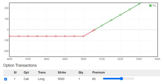
The key to becoming a successful option trader is to select the best strike price and time frame to match your risk profile and goals.
The higher the strike price of a call, the premiums are lower. And lower the delta, the greater is the leverage. At-the-money (ATM) and Out-of-the-money (OTM) options seem lucrative for option buyers.
Short Call
Secondly, let us understand a ‘Short Call.’
A short call involves the selling of a call option. It is a slightly bearish and neutral strategy.
The strategy has limited reward potential and unlimited risk.
A short call strategy has a positive pay–off when there is a fall in the underlying stock or volatility contraction. The strategy has a negative pay-off when there is an increase in the underlying stock, or volatility expansion.
Normally it’s advisable for traders to sell the call at a strike price which is greater than the current market price of the underlying asset i.e. Selling an Out of the Money (OTM) call.

Below is the illustration of the payoff diagram of a Short Call Option:
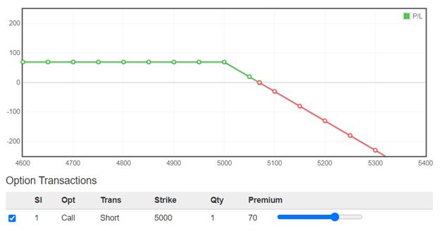
The key incentive of selling a call is that you can profit under three scenarios:
- when the underlying stock declines,
- move sideways,
- or rise slightly
The probability of success in the trade is 2/3rd. An advantage of selling a naked call is that it can be structured to have a higher probability of success than trading the underlying stock or buying a call. A disadvantage to selling any option is that you have unlimited risk if the asset price rises and goes above the strike price.
A call option seller has time on his side and with each passing day, premiums fall considering other factors don’t move much.
Long Put
Since we have already explained a ‘Long Call’ earlier, let us now understand a ‘Long Put.’
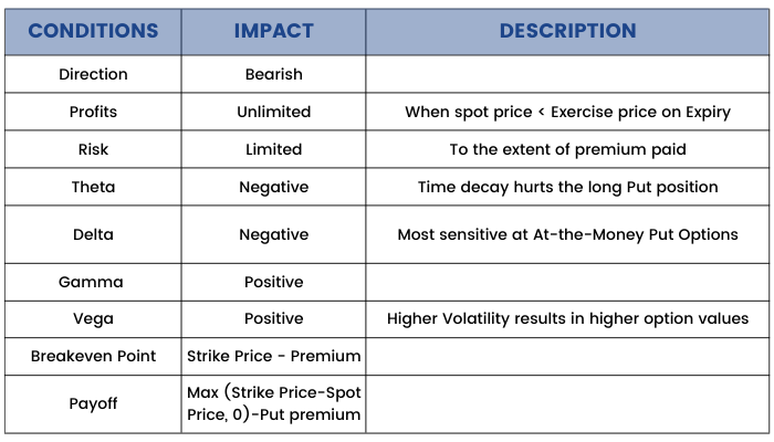
A long put involves buying a put option. It is a bearish strategy. A long put strategy is associated with unlimited profit potential and limited losses or risk to the extent of the premium paid. A trader profits from a long put strategy when the underlying asset falls below the strike price.
A long put normally increases in value from a decline in the underlying stock or volatility expansion. It declines in value from a rise in the underlying stock, time decay, or volatility contraction of the underlying asset.
Unlock the power of options trading with our 'Long Put' masterclass. Elevate your skills and explore 7 profitable strategies today!
Below is the illustration of the payoff diagram of a Long Put Option:
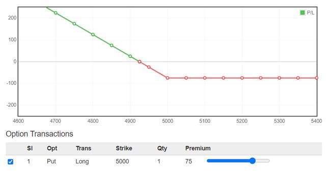
The key to becoming a successful option trader is to select the best strike price and time frame to match your risk profile and goals.
The lower the strike price of a put, the premiums are lower. And the lower the delta, the greater is the leverage. At-the-money (ATM) and Out-of-the-money (OTM) options seem lucrative for put option buyers, when they are bearish on the underlying asset or the overall market.
Short Put
As we have learned a ‘Short Call’ earlier; now, we will discuss a ‘Short Put.’
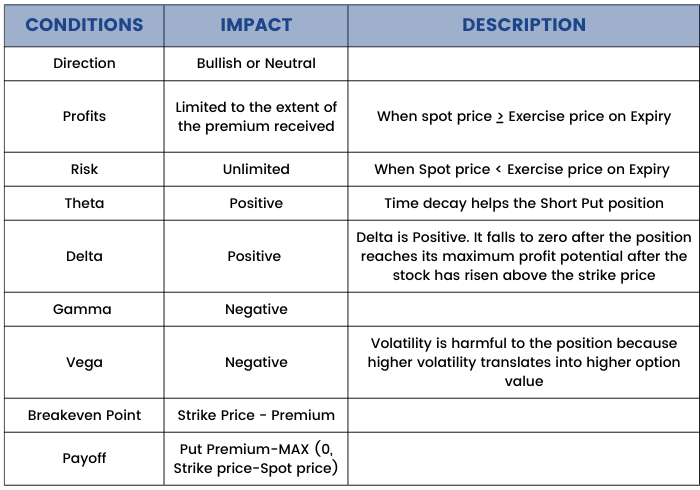
A short put involves the selling of a put option. It is a slightly bullish and neutral strategy. A short put has limited profit potential, which is the premium received and unlimited risk. A short put strategy has a positive pay-out when there is an increase in the underlying stock or volatility contraction. It declines in value from a decline in the underlying stock or volatility expansion.
Below is the illustration of the payoff diagram of a Short Put Option:
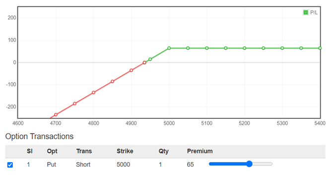
The key incentive of selling a put is that you can profit under three scenarios:
- when the underlying stock rise,
- move sideways,
- or fall slightly
The probability of success in the trade is 2/3rd. An advantage of selling a naked put is that it can be structured to have a higher probability of success than trading the underlying stock or buying a put. A disadvantage to selling any option is that you have unlimited risk if the asset price falls and goes below the strike price.
A Put option seller has time on his side and with each passing day, premiums fall considering other factors don’t move much.
Long Call Vs Short Put
During the study of Long Call and Short Put, we found both are very similar in the thought process, but there are a few differences that we will focus upon in this section.
Long call and a Short put are both bullish strategies. There is a difference between both with respect to the risks involved, and profit potential.
Buying a call is a limited-risk strategy whereas selling a put is an unlimited-risk strategy.
Which strategy is better in the particular circumstance depends on the risk profile of the trader, time frame, and anticipated magnitude of the move.
If the trader is bullish in the short term, then the purchase of a call may be appropriate; however, if the trader is bullish but believes that the underlying stock can fluctuate and the underlying will take time for the bullish move to occur, then selling an Out-of-the-money (OTM) put maybe appropriate.
An important aspect which needs to be kept in mind while deciding whether to buy a call or sell a put is the volatility factor. If an increase in the volatility is expected, then buying call options are always better as while selling a put, the premiums may not decay fast.
Moreover if you want to sell a put, it is always better to initiate it towards the second half of the expiry period. Since the Expiry is near, premium decays are faster.
The table below compares the characteristics of a long call to the characteristics of a short put:

Long Put Vs Short Call
Now we will discuss the differences between a 'Long Put' and a 'Short Call,' both being somewhat similar.
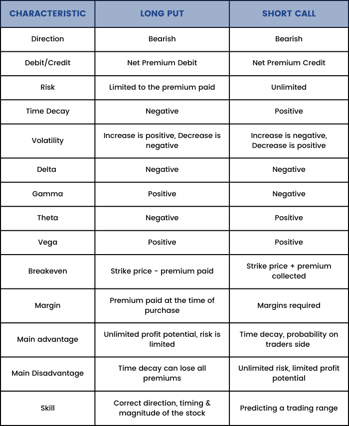
A long put and a short call both are bearish strategies. Even though they both are bearish, they have opposite risks and rewards.
Buying a put is a limited-risk strategy, whereas selling a call is an unlimited-risk strategy.
Which strategy is better in the particular circumstance depends on the risk profile of the trader, time frame, and anticipated magnitude of the move.
If the trader is bearish in the short run, then the purchase of a put may be appropriate; however, if the view is bearish but believe that the underlying stock can fluctuate and that it will take time for the bearish move to occur, then selling an Out-of-the-money (OTM) call may be appropriate.
An important aspect which needs to be kept in mind while deciding whether to buy a Put or sell a Call is the volatility factor. If an increase in the volatility is expected, then buying Put options are always better as while selling a Call, the premiums may not decay fast.
Moreover if you want to sell a Call, it is always better to initiate it towards the second half of the expiry period. Since the Expiry is near, premium decays are faster.
The table below compares the characteristics of along put to the characteristics of a short call:
Bull Spread Strategy
As we have discussed earlier there are four types of Option Spread Strategies:
- Bull Spread
- Bear Spread
- Ratio Backspread
- Ratio Front Spread
Firstly, we will start off with: ‘Bull Spread’ strategy.
Whether we analyse a stock through fundamentals or technical, it’s extremely important for us to know how to trade that analysis. What trade action to be taken which will minimise our risk and maximise our profit and hence achieving a good risk reward ratio.
The spread strategies are one of the simplest option strategies that a trader can implement. Spreads are multi leg strategies involving two or more options. By the term multi leg strategies, we mean that the strategy requires two or more option transactions.
They are initiated when we have a bullish or a bearish stance in the underlying, but the extent of bullishness or bearishness is not very high.
It is devised when your outlook on the stock/index is ‘moderate’ Bullish and not really ‘aggressive’. A Bull spread can be initiated with either calls or Puts.
Spread strategies help the traders to achieve the following:
1. Protect the downside (in case you are proved wrong)
2. The amount of profit made is also predefined (capped)
3. As a trade off since the trader is capping profits, he gets to participate in the market for a lesser cost.
Bull Spread strategy using Calls
Let us first discuss a bull spread using calls.
The bull call spread is a two leg spread strategy which involves trading in At the money (ATM) and Out of the Money (OTM).
To implement a Bull Call Spread Strategy–
1. Buy 1 AT-THE-MONEY (ATM) Call option (leg 1)
2. Sell 1 OUT OF-THE-MONEY (OTM) Call option (leg 2)
When you do this, one needs to ensure –
1. All strikes belong to the same underlying
2. Belong to the same expiry series
Example:
A trader is bullish on NIFTY. He decides to go long on 17350 strike call option by paying a premium of 111 and he expects that it will not go above 17450, so he takes a short call option and receives a premium of 64.
Nifty Spot is trading at 17360
The net cash flow is the difference between premium the trader receives and pay i.e. (111 - 64) = 47
Option Chain:

In a bull call spread there is always a ‘net debit’ of premium. The trader pays the premium net, after we initiate the trade, the market can move in any direction. Therefore let us take up a few scenarios to get a sense of what would happen to the bull call spread for different levels of expiry.
The payoff for various prices are as follows:

Maximum Loss: Net Premium Outflow 47
Maximum Profit: Spread- Max Loss 53
Breakeven Point: Lower Strike + Max Loss 17397
As we can see from the above example, the loss and profit are both limited. Maximum profit the strategy can generate is 53 and maximum loss is 47.

We can say that the bull call spread is a great alternative to simply buying a call outright: keeping in mind when the trader is not aggressively bullish in the underlying stock. The bull call spread reduces the breakeven price and decreases the capital required to be bullish on a stock, it also is a strategy that takes into consideration realistic expectations.
The volatility of the underlying asset should increase for the strategy to generate profit.
Bulls Spread Strategy using Puts
A Bull Put spread is again a bullish spread strategy which is implemented when the trader is mildly bullish on the underlying asset. It is devised similar to a bullish call spread but instead of using calls, we use puts instead.
It involves buying a put at a lower strike price and selling a put at a higher strike price i.e. the put which you go long in is Out of the Money (OTM) put option and the Put you sell is In the money (ITM) or At the money (ATM) Put Option.
We basically have a net credit of premium, when the strategy is implemented. This net credit premium will be the maximum profit of the strategy.
The maximum loss of the strategy is also limited to the extent of spread minus the maximum profit of the strategy.
We must remember that whenever we are devising such strategies the underlying volatility of the strategy should increase, for the strategy to give profit.
If the underlying asset doesn’t move and the volatility doesn’t increase in the desired direction of the trader (which is bullish) the trader will end up making a loss.
We take the same example as above and devise a bullish spread using Puts.

Maximum Loss: Spread-Max Profit 48
Maximum Profit: Net Premium Inflow 52
Breakeven Point: Lower Strike+Max Loss 17398

As can be seen from the example above the loss and profit are both limited. Maximum loss from this strategy is 48 and minimum profit is 52.
To conclude, we can say that bull spread can be initiated by either calls or puts. The Underlying Volatility should increase. Calls will have a net premium debit whereas using puts will result in a net premium credit.
Bear Spread Strategy
Secondly, let us understand a ‘Bear Spread Strategy.’
The Bear Spread is quite easy to implement, similar to the bull spread strategy. This can also be devised both with Calls and Puts.
One would implement a Bear spread when the market outlook is moderately bearish, i.e. you expect the market to go down in the near term while at the same time you don’t expect it to go down much.
A spread strategy as we know limits both profits and losses as it involves buying and selling of options of the same category but different strike prices.
Bear Spread using Puts
A risk averse trader would implement Bear Put Spread strategy by simultaneously –
- Buying an In the money Put option
- Selling an Out of the Money Put option
There is no compulsion that the Bear Put Spread has to be created with an IN-THE-MONEY (ITM) and OUT OF-THE-MONEY (OTM) option. The Bear Put spread can be created employing any two put options. The choice of strike depends on the aggressiveness of the trade. However, an important thing to be kept in mind while devising the strategy is - Both the options should belong to the same expiry and same underlying.
A bear put spread is established for a net debit (or net amount of premium paid) and this strategy will profit when the underlying volatility of the stock increases and the stock price also decreases.
Example
A trader is bearish on NIFTY. He sells a Put of Strike Price 17350, receiving a premium of 95 and buys a put of strike 17450 by paying a premium of 147.
Nifty spot price is currently trading at 17360
Option Chain:


Maximum Loss: Net Premium Outflow 52
Maximum Profit: Spread- Max Loss 48
Breakeven Point: Higher Strike- Max Loss 17398

As can be seen from the example above the loss and profit are both limited. Maximum loss from this strategy is 52 and maximum profit is 48. The trader would start incurring losses if the price of the underlying asset increases i.e. inverse to what he has been speculating. The volatility of the underlying stock should increase for the strategy to generate profits.
Bear Spread using Calls
As we know spread strategy involves buying and selling options of the same category but different strike prices. Bear call spread involves:
Selling a call at a lower strike price i.e. an In the Money option / At the Money option and Buying a call at a higher strike price i.e. Out of the Money Options.
A bear call spread is established for a net credit (or net amount of premium received) and profits from a declining stock price or passage of time.
Example.
Sell a Call of Strike Price 17350, receiving a premium of 111 and buy a call of strike 17450 by paying a premium of 64.

Maximum Loss: Spread- Max profit 53
Maximum Profit: Net Premium Inflow 47
Breakeven Point: Higher Strike- Max Loss 17397

As can be seen from the example above the loss and profit are both limited. Maximum loss from this strategy is 53 and maximum profit is 47. The trader would start incurring losses if the price of the underlying asset increases i.e. inverse to what he has been speculating.
We can say that the bear spread is a great alternative to simply buy a put out right. It can be initiated by either calls or puts. The Underlying Volatility should increase. Calls will have a net premium credit whereas using puts will result in a net premium debit, keeping in mind when the trader is neutral to bearish on the price action in the underlying stock.
Call Ratio Back Spread Strategy
Next, we will learn a ‘Call Ratio Back Spread Strategy.’
Ratio strategies are special types of strategies which are devised when we don’t want to pay a time value of options.
Let’s break the name of the strategy Call Ratio Back spread and understand what does it mean and imply.
Ratio Spread strategy – can be broken in 2 parts. Ratio and spread.
Spread as we have already discussed before, means simultaneously buying and selling of options of the same category but at different strike price and same expiry.
Ratio means that when these buying and selling of options are done in a particular ratio. i.e. trading different quantities of calls or puts.
Assume we buy calls – say 1 lot and simultaneously sell calls – maybe 2 lots. We are basically buying and selling options simultaneously of the same category but different quantities.
When do we initiate a Call Ratio Back spread strategy?
This strategy is initiated when we have a view on the underlying in addition to the volatility expectation about the market. Volatility judgement plays a key role in the success of this strategy.
The Call Ratio Back Spread is a 3 leg option strategy. It involves
- Buying 2 OUT OF-THE-MONEY (OTM) call option
- Selling 1 IN-THE-MONEY (ITM)/ AT-THE-MONEY (ATM) Call option.
2:1 ratio is the classic ratio followed, However we can use multiples of the same. It means 2 options bought for every one option sold, or 4 options bought for every 2 options sold, so on.
This strategy should be devised when the trader is:
- Very Bullish on the underlying asset.
- Volatility is expected to increase to a great extent.
The Payoff from the strategy:
- Unlimited profit if the market goes up
- Limited profit/ or loss if market goes down
- A predefined loss if the market stay within a range
So to make money by this strategy the market has to move big.
Usually, the Call Ratio Back Spread is deployed for a ‘net credit’ or net inflow of premium. The ‘net credit’ is what we make if the market goes down, as opposed to our expectation of the market going up.
On the other hand if the market indeed goes up, then we make an unlimited profit.
Example
Assume Nifty Spot is at 16743 and you expect Nifty to hit 17100 by the end of expiry. This is clearly a bullish outlook on the market.
To implement the Call Ratio Back Spread –
1.Sell 1 lot of 16600 CE (ITM)
2.Buy 2 lots of 16800 CE (OTM)
We need to make sure that –
1.The Call options belong to the same expiry
2.The Call options belong to the same underlying
3.The ratio of the strategy is maintained
16600 CE, one lot short, the premium received for this is ₹201/-
16800 CE, two lots long, the premium paid is ₹78/- per lot, so ₹156/- for 2 lots
Net Cash flow is = Premium Received – Premium Paid i.e. 201 – 156 = 45 (Net Premium Inflow )
With these trades, the call ratio back spread is executed. Let us check what would happen to the overall cash flow of the strategies at different levels of expiry.


So we see, as the market goes up, so do the profits, but when the market goes down, you still make some money, although limited.
Important pointers of the strategy which we can see here are:
- Spread = Higher Strike – Lower Strike
16800 – 16600 = 200 - Net Premium Inflow= Premium Received for lower strike – 2*Premium of higher strike
201 – (2*78) = 45 - Max Loss = Spread – Net Premium Inflow
200 – 45 = 155 - Max Loss occurs at Higher Strike.
16800 - Max Profits =Unlimited as the prices rise above the higher strike price
- Lower Breakeven = Lower Strike + Net Premium Inflow
16600 + 45 = 16645 - Upper Breakeven = Higher Strike + Max Loss
16800 + 155 = 16955
Volatility increase in the underlying is good for this strategy. When you are extremely bullish in an underlying or any news upcoming, then this strategy will give good returns.
Put Ratio Back Spread Strategy
After covering the 'Call Ratio Back spread strategy' in the last unit, next, we will learn the 'Put Ratio Back Spread Strategy.'
The Put ratio back spread is similar except that the traders view is bearish on the market or stock.
When do we initiate a Put Ratio Back spread strategy?
This strategy is initiated when we have a view on the underlying in addition to the volatility expectation about the market. Volatility judgement plays a key role in the success of this strategy.
The Put Ratio Back Spread is a 3 leg option strategy. It involves
- Buying 2 OUT OF-THE-MONEY (OTM) Put option
- Selling 1 IN-THE-MONEY (ITM)/ AT-THE-MONEY (ATM) Put option.
Note: All the options should be of the same underlying and same expiry.
2:1 ratio is the classic ratio followed, however we can use multiples of the same. It means 2 options bought for every one option sold, or 4 options bought for every 2 options sold, so on.
This strategy should be devised when the trader is:
- Very Bearish on the underlying asset.
- Volatility is expected to increase to a great extent.
When we implement the Put Ratio Back Spread we have:
- Unlimited profit if the market goes down
- Limited profit if market goes up
- A predefined loss if the market stays within a range
We make money as long as the market moves in either direction, of course the strategy is more favourable if the market goes down.
Example:
Nifty Spot is at 16506 and you expect Nifty to hit 16000 by the end of expiry. This is clearly a bearish expectation.
To implement the Put Ratio Back Spread:
- Sell 1 lot of 16500 PE (IN-THE-MONEY (ITM)) @134
- Buy 2 lots of 16200 PE (OUT OF-THE-MONEY (OTM)) @ 46
- Net Cash flow is = Premium Received – Premium Paid i.e. 134 – 92 = 42
Let us check what would happen to the overall cash flow of the strategies at different levels of expiry.

Important pointers of the strategy which we can see here are:
- Spread = Higher Strike – lower strike
16500 – 16200 = 300 - Max loss = Spread – Net Premium Inflow
300 – 42 = 258 - Max Loss occurs at = Lower strike price
- Lower Breakeven point = Lower strike – Max loss 16200 – 258 = 15942
- Upper breakeven point = Lower strike + Max loss
16200 + 258 = 16458
Volatility increase in the underlying is good for this strategy. When you are extremely bearish in an underlying or any news upcoming, then this strategy will give good returns.
Hedging Strategy - Covered Call
Earlier, we learned that there are two types of hedging strategies, namely ‘Covered Call’ and ‘Protective Put.’ Let us now discuss them in detail, starting off with the 'Covered Call' in unit. But before that, we must understand what exactly is 'Hedging?'
Hedging is a technique that is frequently used by many investors and options traders. The basic principle of hedging is that it is used to reduce or eliminate the risk of holding one particular investment position by taking another position.
Hedging doesn’t help the trader or an investor to make money. It helps them to protect themselves from a probable loss. The versatile nature of options make them useful when it comes to hedging.
Many investors that don’t usually trade options use them to hedge against existing investment portfolios of stock. There are few options trading strategies that can specifically be used for this purpose, such as covered calls and protective puts.
What is a 'Covered Call' ?
A covered call is an options strategywhereby an investor holds a long position in a stock either in Cash or Futures and sells call options on that same stock in an attempt to generate increased income from the asset or to protect downside to a certain extent.
This is often employed when an investor has a short-term neutral view on the stock and for this reason holds the stock long and simultaneously has a short position via the option to generate income from the option premium.
It serves as a short-term small hedge on a long stock position and allows investors to earn premium, hence reducing costs.
Strategy Involves:
1.Buy Stock ( futures or Cash )
2.Sell 1 Call Option
The breakeven point of the strategy will be Current stock price minus the premium received for selling the call.
Maximum Profit is limited, strike price minus the current stock price plus the premium received for selling the call.
And what is the maximum loss? The trader receives a premium for selling the option, but most downside risk comes from owning the stock, which may potentially lose its value, if the asset goes down. In fact, selling the option creates an “opportunity risk.” i.e. if the stock price skyrockets, the calls might be assigned and the trader will miss out on those gains. As a call is sold at a higher strike price the loss from call sold will be offset by stock as the price rises.
A covered call can enable you to profit in a sideways market; take advantage of an anticipated decline in volatility. If you already own stock, and volatility in the market rises dramatically, you may want to consider selling a covered call because the option premium may be attractive and you can profit from a decline in volatility (theta). If implied volatility declines after the call is sold, assuming that all other factors remain constant, a call option will decrease in value.
Hedging Strategy – Protective Put
The next hedging strategy that we will discuss here is ‘Protective Put.’
Successful investors are concerned with managing risk effectively while they focus on maximizing returns. The main goal for investors should be maximizing risk-adjusted returns rather than total returns.
Options provide a great way to help manage risk with their tremendous flexibility and controllable costs. Protective put strategy helps in protecting the portfolio by incurring a minor cost. This strategy is widely used to help limit downside risk.
Protective put is a hedging strategy where the holder of a security buys a put to guard against a drop in the stock price of that security, which he already holds. This can also be applied to a basket of securities or portfolio. In case the trader wants to hedge the entire portfolio, an equivalent amount of Index puts can be bought.
It basically involves going long on a stock (either in cash segment or in futures) and simultaneously buying a put to limit the downside.
There is unlimited profit potential in this strategy. The protective put is also known as a synthetic long call as its risk/reward profile is the same as that of a long call.
The formula for calculating profit is given as:
- Maximum Profit = Unlimited
- Profit Achieved When Price of Underlying > Purchase Price of Underlying + Premium Paid
- Maximum loss for this strategy is limited and is equal to the premium paid for buying the put option.
- Max Loss Occurs When Price of Underlying <= Strike Price of Long Put
- Breakeven Point = Purchase Price of Underlying + Premium Paid
Collar Strategy
From this section onwards, we will start with different volatility and range-bound strategies. First, let us begin with the understanding of a ‘Collar Strategy.’
A collar strategy is a combination of a covered call and a protective put. It can be devised by
- Buying the stock ( either cash or futures)
- Selling out of the money call
- Buying out of the money Put
This strategy limits the return of the stock or the portfolio to a specified range and can hedge a position against the volatility of the underlying asset.
If the stock rises, this strategy performs like a covered call. If the stock declines, this strategy limits the loss at the put strike price
- A collar strategy limits both gains and losses.
- The payoff from the strategy is similar to a Bull Call Spread
- Collars may be used when investors want to hedge a long position in the underlying asset from short-term downside risk.
Option Chain:


We can see that if the stock rises, this strategy performs like a covered call. If the stock declines, this strategy limits the loss at the put strike price.
Unlock success in options trading with our 'Collar Strategy' masterclass. Elevate your skills and profits today!
Straddle
Next, we will learn a 'Straddle' Strategy, which can be 'Long Straddle' or a 'Short Straddle.' Let us discuss both of them in this section.
Many times we have been in a situation where we initiate a trade after all our conviction and study, either on the buy or sell side and right after we initiate the trade the market moves just the other way round! Yes, most of us have been in this situation many times. All our strategy, planning, efforts, and capital goes for a toss whenever such kinds of situations arise.
In fact this is one of the primary reasons why most professional traders go beyond the regular directional based trades and set up strategies which are insulated against the unpredictable market direction.
Strategies whose profitability does not really depend on the market direction are called “Market Neutral” strategies.
Let us understand some of the market neutral strategies and how a regular retail trader can execute such strategies.
Let us begin with a ‘Long Straddle.
A long straddle is perhaps the simplest market neutral strategy to implement. Once implemented, the Profit & Losses are not affected by the direction in which the market moves. The market can move in any direction, but the point is that it has to move. As long as the market moves (irrespective of its direction), profit is generated. The increase in the volatility of the underlying asset will ensure that the strategy generates a positive pay-out.
A Long straddle is created by:
Buy a Call option and Buy a Put option at the same strike price.
Important point to be kept while initiating a long straddle: Both the options belong to the same underlying, the same expiry and the same strike.
Example:
Option Chain:


Maximum Loss: Net Premium Outflow 206
Maximum Profit: Unlimited as price rises or falls
Upper Breakeven Point: Strike price + Maximum Loss 16556
Lower Breakeven Point: Strike price-Maximum Loss 16144

This strategy is quite straightforward to understand and implement.
The trader simply buys calls and puts, each leg has a limited downside, hence the combined position also has a limited downside and an unlimited profit potential. It is like placing a bet on the price action each. The direction does not matter here.
But let’s think it over again– if the direction does not matter, what matters for this strategy? Do we always end up making money in this strategy as the market will move in some direction?
The Answer is Volatility!!
Volatility plays the key role when we implement the straddle. A fair assessment on volatility serves as the backbone for the straddle’s success.
Two things are important for a straddle to generate profits. They are as follows:
1.Theta Decay – All else equal, options are depreciating assets and it particularly hurts long positions. The closer we get to expiration, the lesser time value of the option. Time decay accelerates exponentially during the last week before expiration.
2.Large break-evens – In the example we discussed, the breakeven points are almost 200 points away from the AT-THE-MONEY (ATM) strike. The lower breakeven point was 16144 and the upper breakeven was 16556, considering the AT-THE-MONEY (ATM) strike was 16350. The market has to move approx. 2% (either ways) to achieve breakeven. This means that from the time we initiate the straddle, the market or the stock has to move at least 2% on either ways for us to start making money and this move has to happen within a maximum of the expiry of the contract.
Such a large move is quite a challenge in normal scenarios. Keeping the above two points plus the volatility factor, we can summarize what really needs to work in your favor for the straddle to be profitable –
1.The volatility should be relatively low at the time of strategy execution
2.The volatility should increase during the holding period of the strategy
3.The market should make a large move – the direction of the move does not matter
4.The expected large move is time bound, should happen quickly – well within the expiry
Long straddles are to be set around major events, and the outcome of these events to be drastically different from the general market expectation.
Short Straddle
To initiate a short straddle, instead of buying the AT-THE-MONEY (ATM) Call and Put options (like in long straddles) we just have to sell the AT-THE-MONEY (ATM) Call and Put option. When you sell the AT-THE-MONEY (ATM) options, you receive the premium in your account.
The short straddle works exactly opposite to the long straddle. Short straddles work best when markets are expected to be in a range and not really expected to make a large move.
Many traders fear short straddle considering the fact that short straddles have unlimited losses on either side. However, from my experience, short straddles work really well if you know how exactly to deploy this, keeping in mind Theta, volatility, and event occurrence.
Example:

Maximum Loss: Unlimited as price rises or falls
Maximum Profit: Total Premium Received 206
Upper Breakeven Point: Strike price + Maximum Loss 16556
Lower Breakeven Point: Strike price - Maximum Loss 16144

Strangle
If you have understood the straddle, then understanding the ‘Strangle’ is quite straightforward. For all practical purposes, the thought process behind the straddle and strangle is quite similar. Strangle is an improvisation over the straddle, mainly to reduce the cost of implementation.
In a Long straddle you are required to buy call and put options of the AT-THE-MONEY (ATM) strike. However the long strangle requires you to buy Out of The Money (OTM) call and put options. Remember when compared to the AT-THE-MONEY (ATM) strike, the OUT OF-THE-MONEY (OTM) will always trade cheap, therefore this implies setting up a strangle is cheaper than setting up a straddle.
Few points to be kept in mind while initiating a long strangle are the same as initiating a long straddle. They are:
1.The volatility should be relatively low at the time of strategy execution
2.The volatility should increase during the holding period of the strategy
3.The market should make a large move – the direction of the move does not matter
4.The expected large move is time bound, should happen quickly – well within the expiry
5.Long strangle is to be set up around major events, and the outcome of these events have to be drastically different from the general market expectation.
Long Strangle
Option Chain:

Nifty Spot is trading at 16360. We Buy 1 Call and 1 Put Out of the money strike prices. Call at 16450 strike price at 64 and Put at 16250 strike price at 95 premiums respectively. Total premium which we pay to implement this strategy is 64+59 = 123. This means to be in profit from this strategy the underlying asset has to move 123 points up or down from 16360 for the trader to generate returns.

Maximum Loss: Net Premium Outflow 123
Maximum Profit: Unlimited as price rises or falls
Breakeven Point 1: Call Strike Price + Maximum Loss 16573
Breakeven Point 2: Put Strike Price - Maximum Loss 16127

When we buy calls and puts, it has a limited downside, hence the combined position also has a limited downside to the extent of the premium paid and an unlimited profit potential on movement of upside or downside direction of the asset. So, a long strangle is like placing a bet on the price action each-way– you make money if the market goes up or down, keeping in mind an increase in volatility.
Short Strangle
Now let us consider a short strangle. This is just the opposite to buying a strangle. Instead of buying Calls and put, here we sell calls and puts both Out of the money and receive premiums. The maximum profit which can be generated from this strategy is limited to the extent of the premium received. Once the price movement goes beyond the range, we start incurring a loss.
Since we are selling out of the money options, the premium received is lower, but the range increases which cushion the trader against the sudden movement of the asset. What needs to be kept in mind is that at the time of executing the strategy, there must be Volatility.
The volatility in this case needs to reduce during the holding period and should be high at the time of execution of the contract. The trader bets against the volatility to make money from this strategy. If the trader identifies a specific range in which the stock is expected to trade, and no major events are round the corner, a short strangle is a perfect strategy to execute.
Example: Short Strangle
Nifty Spot is trading at 16360. We Sell 1 call and 1 put Out of the money strike prices. Call at 16450 strike price at 64 and Put at 16250 strike price at 95 premiums respectively. Total premium which we receive when the strategy is implemented is 64+59 = 123. This means to be in profit from this strategy the underlying asset has to stay in the range of 123 points up or down from 16360.

Maximum Loss: Unlimited as price rises or falls
Maximum Profit: Total Premium Received 123
Breakeven Point 1: Call Strike Price + Maximum Profit 16573
Breakeven Point 2: Put Strike Price - Maximum Loss 16127

Strip Strategy
The strip strategy is a modified, and a more bearish version of the straddle strategy. It involves buying a particular number of At-the-money calls and twice the number of puts.
We must remember that the Calls and Puts must be of the same underlying stock, strike price and expiration date.
Let’s know how do we construct a Strip Strategy:
1. Buy 1 Call AT-THE-MONEY (ATM)
2. Buy 2 Puts AT-THE-MONEY (ATM)
We use this strategy when we expect volatility to increase in the near future and market direction to be on the bearish side. Large profit is attainable with the strip strategy when the underlying stock price makes a strong move either upwards or downwards at expiration, but gains are made faster and larger if the movement of the underlying is on the downside. The risk is limited to the net premium paid for the position and the maximum profit is unlimited.
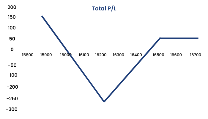
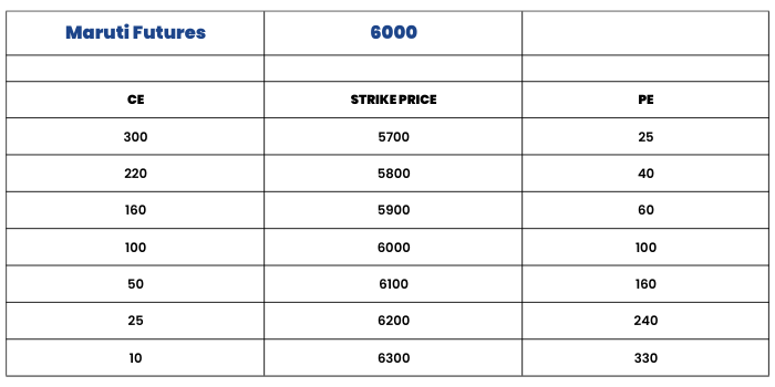
Example:
Consider Maruti Futures which is trading at Rs 6000. We Buy a Call of 6000 strike price @ ₹100 and simultaneously buy 2 puts of strike 6000 @ ₹100 each. Both Calls and Puts should be of the same expiry date.
1C+ @ 6000 = 100
2P+ @ 6000 = 100
Option Chain:

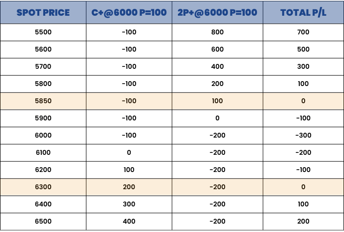

Maximum Profit : Unlimited
Maximum Loss : Limited to the net Premium Paid = 300
Lower Break-even Point = Strike price – (net premium paid/2) = 6000 - (300/2) = 5850
Upper Break-even Point = Strike price + net premium paid = 6000 + 300 = 6300
The Volatility should increase after devising the strategy to generate positive payoffs.
Strap Strategy
The strap strategy is a modified and bullish version of the straddle strategy. It involves buying more At-the-money calls and lesser puts.
We need to make sure that both the calls and puts should be of the same underlying stock, strike price and expiration date.
We conduct a strap strategy by:
1. Buy 2 Call AT-THE-MONEY (ATM)
2. Buy 1 Puts AT-THE-MONEY (ATM)
We use this strategy when we expect volatility to increase in the near future and market direction to be on the bullish side. Large profit is attainable with the strap strategy when the underlying stock price makes a strong move either upwards or downwards at expiration, but gains are made faster and larger if the movement of the underlying is on the upside. The risk is limited to the net premium paid for the position and the maximum profit is unlimited.
The most important thing for all these strategies, i.e. Straddle, Strangle, Strip and Strap is Volatility. The market has to make big moves in order for these strategies to make money for you.
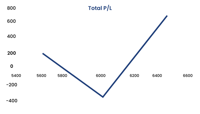
Strap strategy
Option Chain:
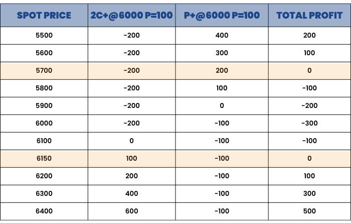
Maximum Profit : Unlimited
Maximum Loss : Limited to the net Premium Paid = 300
Upper Break-even Point = Strike price + (net premium paid/2) = 6000 + (300/2) = 6150
Lower Break-even Point = Strike price - net premium paid = 6000 - 300 = 5700
Butterfly Strategy
Now, we will learn to implement a ‘Butterfly Strategy,’ which is a fairly complex strategy compared to other strategies that we have learned earlier. So let us begin.
A butterfly spread is a neutral option strategy combining bull and bear spreads together. It is a four legged strategy- which means the trader has to take positions in four different option contracts to implement this strategy.
The trader implements these four option contracts with the same expiration in three different strike prices.
One of the unique features of this strategy is that we can implement this by either using Calls or Puts
Let us first discuss it using Calls.
When do we implement butterfly strategy?
A Long Call Butterfly is implemented when the trader is expecting slight or no movement in the underlying asset. The motive behind initiating this strategy is to rightly predict the stock price till expiration and gain from time value of an option premium by undertaking limited risk.
When the trader expects the underlying asset to trade in a narrow range and remain neutral on the direction front, then this strategy is ideal to be implemented.
Remember when we discussed Short Strangle or Short Straddle, we had the view that underlying asset will be in range bound, and the profit occurs if it remains in the range else we start incurring unlimited losses. On the contrary the advantage of a butterfly strategy is that, here the potential risk is also limited.
This is a neutral strategy used for range bound markets and is undertaken during last few days or second half of the expiry to capitalize the time value of Premium.
How to construct a Long Call Butterfly?
A Long Call Butterfly can be created by:
- Buy 1 IN-THE-MONEY (ITM)Call
- Buy 1 OUT OF-THE-MONEY (OTM)Call
- Selling 2 AT-THE-MONEY (ATM)Calls.
We need to make sure that –
- The Call options belong to the same expiry
- All the option contracts belong to the same underlying asset.
- The strike prices are equidistant from each other, i.e. the difference between IN-THE-MONEY (ITM) , OUT OF-THE-MONEY (OTM) and AT-THE-MONEY (ATM) should all be same.
- All the legs of the strategy should be initiated simultaneously.
Example:
Option Chain:


Strategy: Buy 1 (ITM) Call, Sell 2 (ATM) Call and Buy 1 (OTM) Call
Market Outlook: Neutral on the market direction
Spread: Equidistant 100
Lower Breakeven: Lower Strike Price of buy call + Net Premium Paid 16220
Upper Breakeven: Higher Strike Price of buy call - Net Premium Paid 16380
Maximum Loss: Limited to Net Premium Paid 20
Maximum Profit: Limited and it is achieved when the underlying asset remains at the middle strike price on expiry 16300
Calculation of Maximum Profit (Spread - Premium Paid) 80
Now let us discuss a Long Butterfly strategy using Puts:
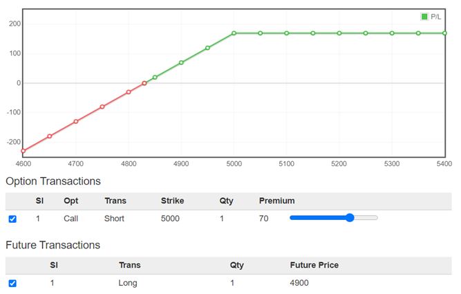
A long butterfly strategy can be implemented either by calls or Puts! The payoff from the strategy will be the same. The reason behind this is that we can create simple strategies using synthetic positions.
How synthetic options can be used to create a butterfly strategy using Puts?
A Long Butterfly strategy can be devised by:
- Buy 1 IN-THE-MONEY (ITM) Call,
- Sell 2 AT-THE-MONEY (ATM) Call
- Buy 1 OUT OF-THE-MONEY (OTM) Call
- All strike prices to be equidistant
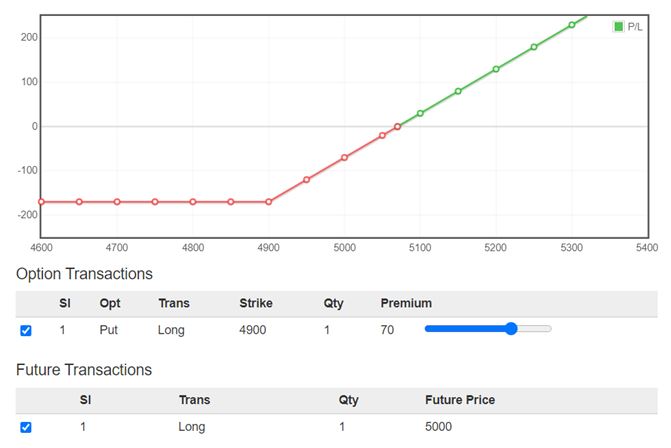
Now one Long call synthetically can be created by Buying 1 put Option and simultaneously Buying 1 Lot of Futures contract (P+ and F+)
Short Call synthetically can be created by Selling 1 Lot of Put and simultaneously selling 1 Lot of Futures Contract. (P- and F-)
So we can re- write the Long Butterfly strategy using calls as:
C+ IN-THE-MONEY (ITM) = P+ , F- IN-THE-MONEY (ITM)
C+ OUT OF-THE-MONEY (OTM) = P+ , F- OUT OF-THE-MONEY (OTM)
2C- AT-THE-MONEY (ATM) = 2 P- , 2 F + AT-THE-MONEY (ATM)
If we solve the above equations, we are net 2 contracts of futures - Buy and simultaneously 2 Lots futures - Sell
Both the above futures lots get cancelled.
Final Equation:
Buy 1 IN-THE-MONEY (ITM) Put , Sell 2 AT-THE-MONEY (ATM) Put and Buy 1 OUT OF-THE-MONEY (OTM) Put
We need to make sure that –
- The Put options belong to the same expiry
- Belongs to the same underlying
- The strike prices are equidistant from each other i.e. the difference between IN-THE-MONEY (ITM) , OUT OF-THE-MONEY (OTM) and AT-THE-MONEY (ATM) should all be the same .
Example:
We consider the same Option chain as used in the above example.


Strategy: Buy 1 (ITM) Put, Sell 2 (ATM) Put and Buy 1 (OTM) Put
Market Outlook: Neutral on the market direction
Spread: Equidistant 100
Lower Breakeven: Lower Strike Price of Buy Put + Net Premium Paid 16218
Upper Breakeven: Higher Strike Price of Buy Put - Net Premium Paid 16382
Maximum Profit: Limited and it is acheived when the underlying asset remains at the middle strike price on expiry 16300
Calculation of Max. Profit: (Spread - Premium Paid) 82
Modified Butterfly Strategy
A regular butterfly option strategy is a neutral or a non-directional strategy where we can profit if the stock moves in a particular range. However, a modified butterfly is a directional strategy, where we make profit if stock moves in our favor but won’t face losses even if the stock remains sideways. We incur losses only when the stock moves against our favorable direction.
It can be created with only Call options a.k.a Long Butterfly or only Put options a.k.a Short Butterfly. But for this particular module or blog, we will be focusing only on modified butterfly option strategy.
They are of two types:
-
Bullish/Call Butterfly
-
Bearish/Put Butterfly
The main objective of this strategy:
- To make profits from directional movement of the stock
- To protect losses due to theta decay if stock moves sideways
Let’s start with a bullish/Call modified butterfly which consists of 3 legs. They are as follows:
-
Buy +1 ATM/Near OTM Call
-
Sell -2 OTM Call
-
Buy +1 Next OTM Call (not equal strikes)

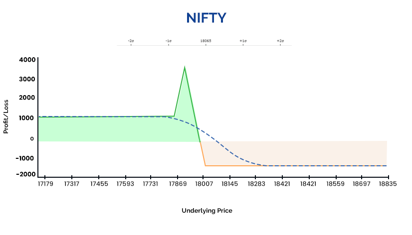
Take a look at the above example, where Buy ATM Call & Selling OTM Calls are of equidistant strikes. However the 3rd leg of buying Far OTM call has been modified with taking a long position 50 points higher rather than 100 points, which makes it a modified butterfly.
Hence one side is completely protected & maximum profit can be realized if it trades in a range bound near the -2 OTM strike that is sold. Loss will only occur below our breakeven point.
Now, let’s discuss a bearish/Put modified butterfly which also consists of 3 legs. They are as follows:
-
Buy +1 ATM/Near OTMPut
-
Sell -2 OTM Put
-
Buy +1 Next OTM Put (not equal strikes)
Take a look at the above example, as the pay-off graph seems exactly opposite to the modified call butterfly. Only difference is the strategy is built with Puts. The view here is bearish. Maximum profit can be realized when price moves in a favorable direction but consolidates near the -2 OTM Strikes which are sold. However, in case it moves further in a favorable direction strategy remains profitable & loss will occur only when it goes above the breakeven point.
Thus, modified butterflies are useful when you wish to create an open ended directional strategy unlike regular butterflies where if the stock moves beyond the range, the strategy incurs loss.
Long Condor Strategy
A Long Condor is similar to a Long Butterfly strategy. The primary difference is that in a butterfly strategy we sell 2 options at a middle strike price, but in a Condor the 2 options which are sold are at separate strikes.
The maximum profit from the condor strategy may be low as compared to a butterfly strategy; but it has a high probability of making money because of the wider profit range.
When to initiate a Long Condor?
A Long Condor spread should be initiated when the trader expects the underlying assets to trade in a narrow range. This strategy benefits from the time decay factor. This strategy can also be devised by using both Calls and Puts as in the case of the butterfly strategy. By using synthetic options concept we use either only Calls or only Puts to device it.
We will discuss the strategy using Calls in our example.
How is the strategy constructed?
A long condor spread is a four-part strategy that is created by buying one Call at a lower strike price, selling one Call with a higher strike price, selling another Call with an even higher strike price and buying one more Call with an even higher strike price. All calls have the same expiration date, and the strike prices are equidistant.
- C+ IN-THE-MONEY (ITM)
- C- AT-THE-MONEY (ATM)
- C- OUT OF-THE-MONEY (OTM) ( Slightly )
- C+ OUT OF-THE-MONEY (OTM) ( Higher )
Example:
Option Chain


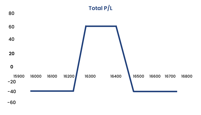
Lower Breakeven: Lowest Strike price + the net premium outflow 16240
Upper Breakeven: Highest Strike price - the net premium outflow 16460
Maximum Loss: Net Premium Outflow 40
Maximum Profit: Difference between Strike Price - Net Premium Outflow 60
So from the above example we can conclude:
Maximum profit is equal to the difference between the strike prices less the net cost of devising the strategy. Maximum profit is realized if the stock price is between the middle strike prices at expiry. In the example above, the difference between the strike prices is 100, and the net cost or the net premium paid for the strategy is 40. The maximum profit is 100 – 40 = 60. This ₹60 can be attained if the spot price on expiry remains between 16300 to 16400.
Maximum risk / Loss: The maximum loss of the strategy is the net premium outflow. Now when does this maximum loss occur?
There are two possible outcomes in which a loss of this amount is incurred by the trader.
If the stock price is below the lowest strike price at expiry, then all calls lapse and expire worthless and the full cost of the strategy i.e. 40 is lost.
On the contrary, if the stock price is above the highest strike price on expiry then all calls are in the money and the condor spread position has a net value of zero at expiry. As a result, the full cost of the position i.e. net premium paid is lost.
There are two breakeven points. The lower breakeven point arises when the stock price equal to the lowest strike price plus the net premium outflow i.e, 16200 + 40 = 16240
The upper breakeven point is the stock price equal to the highest strike price minus the net premium outflow. 16500 - 40 = 16460
So we can conclude:
A long condor spread is the strategy we do when the forecast for underlying is in the range of maximum profit, which is between the middle strike prices of the spread. Long condor spreads profit from time decay; and unlike short straddle and short strangle the potential risk of a long condor spread is limited. It is a variation of the butterfly strategy.
Long condor spreads are sensitive to changes in volatility, should be purchased when volatility is “high” and is expected to decline thereafter.
Conclusion
So, as we conclude this module, learning the theoretical part ends here, but now it is time to implement these option strategies in the market as we saw that there are many options strategies that can be implemented to earn a profit under different market conditions. Yes, it is difficult to have a notion of understanding which strategy to apply under a particular market condition. But such expertise comes with experience.
The most important thing is to learn and understand the market in & out so that no matter what the market condition, you make a handsome profit by the end of the day. In this module, we tried to cover the maximum number of options strategies for you so that you develop your knowledge and become a successful options trader.


